
Motivation and the usual notes
While I was discussing the finer points of my GPU-based vector graphics system, a few friends expressed annoyance with the lack of didactic exposition regarding crucial concepts behind vector graphics, among other things. The primary argument is that most literature assumes, through ignorance, laziness or comfortable complancy, that the mathematics behind Bézier curves are sufficient to present in their final form. Let's fix that.
Passed initial nerd review and is now available to the general public. I'll do some diagrams when I feel like it.
If you asked your typical programmer about Bézier curves, you'd likely find it difficult to differentiate their answer from the general "wisdom" available online, usually on websites with non-existent CSS. In other words, a truckload of circular and poorly motivated reasoning which assumes foreknowledge of the subject to derive it, positing results ahead of the premise. As such, there is little intuition and satisfaction to be gained from any such website, book or programmer. The story of Bézier curves is a fascinating one, and a lot messier than most sources make it out to be. The way they were originally derived is obscured in the publications as a result of the process best illustrated by this hilarious meme masquerading as a paper.
The problem with modern exposition of the subject is that the original spirit of the derivation was obfuscated in favor of an impressive showcase in terms of relations that were uncovered towards the end. As most programmers don't invest much thought in the why and how beyond gaining the ability to use it, nuance is easily lost. As such, "de Casteljau's algorithm" is taken as gospel and statements like "Bézier curves are based on Bernstein polynomials" are common place. They are related to them and are mathematically equivalent, meaning that properties studied on the latter can be used to inform the former. That does not mean they're derived from them or provide any kind of intuition or basis on how to reason about Bézier curves. Their properties are used to prove and generalize what our intuition is implying in simpler cases. To put it differently, there is no clear path to Bernstein polynomials without prior knowledge of the relationship between the two. Otherwise you could say that Bézier curves are based on the binomial distribution and probability theory.
Luckily for you, I am one particularly ridiculous nerd who likes to independently arrive at the constructs he uses in his daily work. So, let us table Bernstein polynomials for now and we'll get back to them organically, once the link arises naturally.
A brief history with some spicy drama
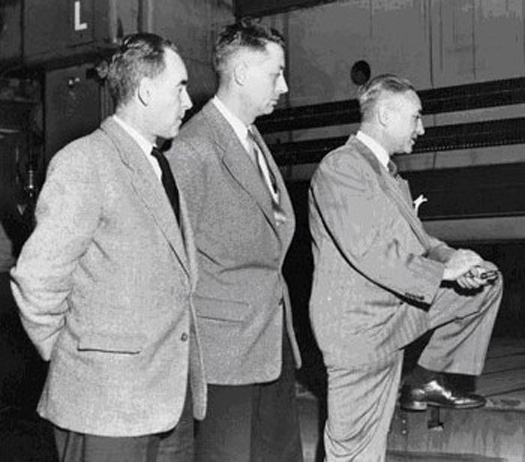 Bézier is the feller in the middle.
It was indeed Pierre Bézier who first popularized the application of these curves in computer aided design of automotive bodies while working at Renault in the 1960s. Renault at the time didn't have a gag order on research disclosure, which allowed Bézier to get his name attached to them under the "I was first to say I was first here" doctrine.
The primary historical reference is still the one by Bézier from a conference at the University of Utah in 1972, a university now famous in the computer graphics community for many contributions to the field and the home of the Newell teapot.
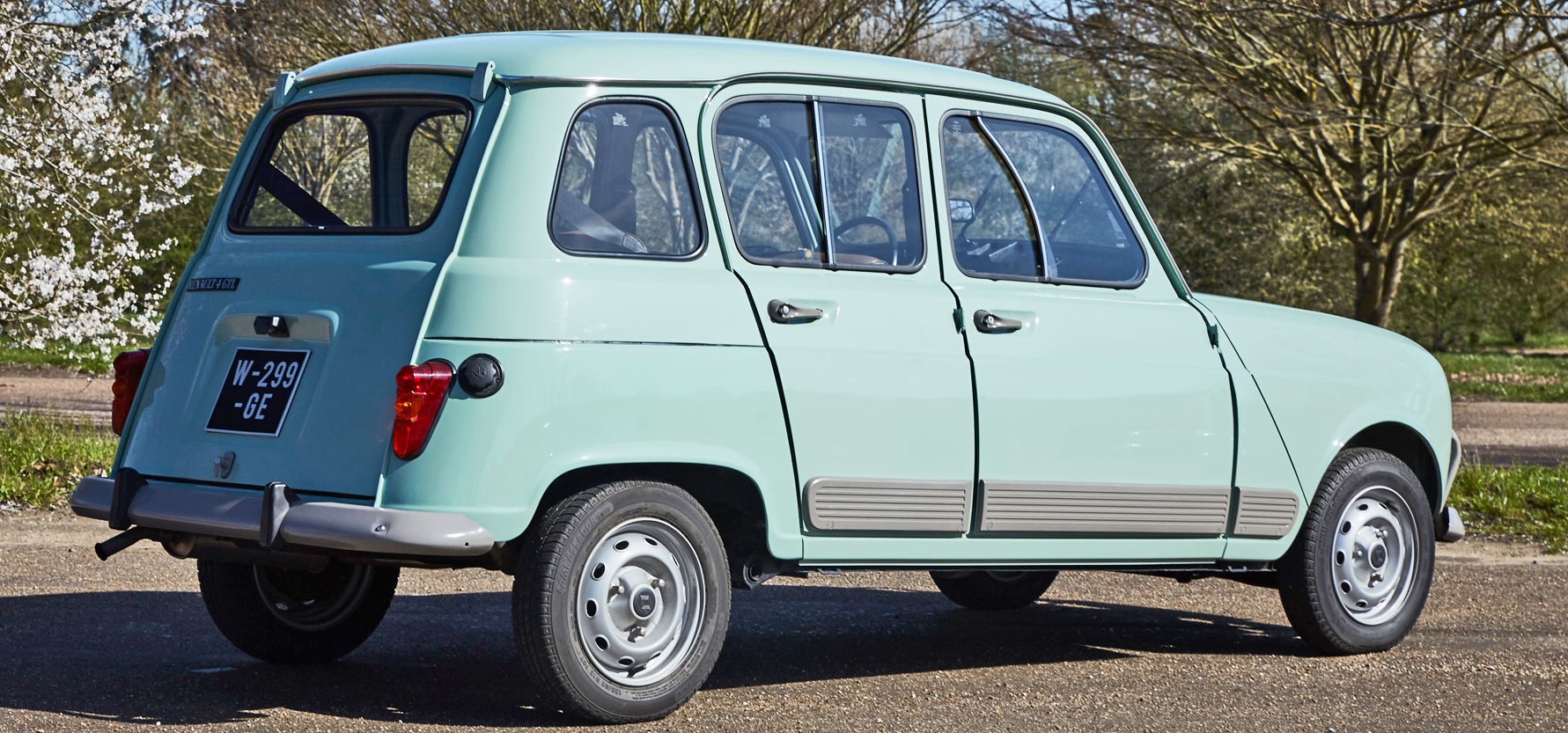 Brought to you by curvy curves.
The thing is... There was another gentleman going by the name of Paul de Casteljau who also worked at a French automotive giant, Citroën... Who claimed to have developed the same curves for the same purpose in the late 1950s, but was barred from publishing his research. Ouch. Now, I am not saying de Casteljau didn't like Bézier much, but he didn't like him. Probably because Bézier patented his life's work. Much like the feud between Newton and Leibniz, a lot of sparks flew here. By the time this was public knowledge, the industry had pretty much associated Bézier with the curves...
The consolation prize attributed to de Casteljau was the "algorithm" used for evaluating the curves. The "algorithm" is merely an unavoidable fact of life, a trivial transformation of the curve equation, and Bézier had to have derived it himself to derive an actionable mathematical basis. While it stings, it's just yet another example of Stigler's law of eponymy, itself a necessity due to the proven possibility of multiple discovery.
Connecting the dots
To achieve anything of note in life, one needs a motivation. One look at curves in analytic geometry and you can see just how much a hassle it is to control/shape the curves intuitively, making our motivation rather clear; finding a way to intuitively control curves as a function of their endpoints and the associated tangent vectors which can be transformed into control points of some sort.
Linear Bézier curve
Our starting point is fundamental analytic geometry and the first construct introduced in analytic geometry is the line. It is fairly trivial to recover a line that goes through two points:
$$\begin{split} y &= \frac{ \mathbf{P}_{1y} - \mathbf{P}_{0y } }{\mathbf{P}_{1x} - \mathbf{P}_{0x}} (x - \mathbf{P}_{0x}) + \mathbf{P}_{0y} \\ &= \frac{ \mathbf{T}_{y} }{\mathbf{T}_{x} } (x - \mathbf{P}_{0x}) + \mathbf{P}_{0y} \\ \end{split}$$
It can be quickly rearranged into a parametric equation as a function of $t$ limited on a $[0,1]$ range:
$$\Large{\begin{split} \mathbf{P}(t) &= \mathbf{P_0} + t(\mathbf{P_1} - \mathbf{P_0}) \\ &= (1-t)\mathbf{P_0} + t\mathbf{P_1} \\ \end{split}}$$
In the context of Bézier curves, this is the linear Bézier curve. Stating the obvious, but it is also the expression for linear interpolation.
The limit of "first principles"
I thought about outlining, in excruciating detail, how one arrives at this parametric line equation. However, if the reader is unable to recover the linear interpolation equation on their own, reading this article may be a premature activity.
Quadratic Bézier curve
Don't get spoiled by the triviality exhibited so far as we're going up a degree. The first proper curve one is introduced to is usually the ubiquitous parabola. Specified in slope-intercept form, it's $y = a_2t^2 + a_1t + a_0$. If you transform it a bit, you get $y = (a_2t + a_1)t + a_0 = a(t)t + a_0$. The parabola is, thus, what happens when you linearly vary the highest degree coefficient of a line (the directional one). Thus, the derivative of a parabola is a line. As a parabola exhibits mirror-symmetry, the derivative at two points on opposite sides will be mirrored (going up, going down). In other words, they are correlated and it is possible to express the tangents as a function of the end points and a third, shared control point.
While we expressed a linear Bézier curve rather intuitively and satisfyingly by linearly interpolating its end points, the quadratic Bézier curve will not yield as easily. It does have a satisfying analogue; we can elegantly express its derivative at any point as a linear interpolation between the two endpoint "velocity vectors" or tangents specified, due to reasons elaborated in the previous paragraph, as $\mathbf{T_0} = \mathbf{P_1} - \mathbf{P_0}$ and $\mathbf{T_1} = \mathbf{P_2} - \mathbf{P_1}$:
$$\Large{\begin{split} \mathbf{P}'(t)/2 &= \mathbf{T_0} + t(\mathbf{T_1} - \mathbf{T_0}) \\ &= (1-t)\mathbf{T_0} + t\mathbf{T_1} \\ \end{split}}$$
If you're not sure why there is a factor of $1/2$ in there, it follows from the fact that the derivative of $x^2$ is $2x$. You have to be mindful of the established rules while we're playing this constructive game. By integrating this and solving for the $c$ (you're right, it's $\mathbf{P}_0$), we recover $\mathbf{P}(t)$:
$$\Large{\begin{split} \mathbf{P}(t) &= 2\int \mathbf{T_0} + t(\mathbf{T_1} - \mathbf{T_0}) \space dt \\ &= 2t\mathbf{T_0} + t^2(\mathbf{T_1} - \mathbf{T_0}) + c \\ &= 2t\mathbf{T_0} + t^2(\mathbf{T_1} - \mathbf{T_0}) + \mathbf{P}_0 \\ \end{split}}$$
And just like that, we have the quadratic Bézier curve. If you swap in the control points, you have a very easy way of evaluating quadratic curves which is sufficient for specifying glyphs of fonts for text rendering. However, to go beyond, one can perform mental gymnastics like the ones we did here. Or we can look for some pattern here. As we have derived the linear Bézier curve as a simple linear interpolation of the end points and the quadratic Bézier curve by noticing its derivative can be expressed in terms of a linear interpolation of the velocity vectors... It just might lead to some generalization if we unroll everything and try to rearrange a bit:
$$\begin{split} \mathbf{P}(t) &= \mathbf{P}_0 + 2t(\mathbf{P_1} - \mathbf{P_0}) + t^2(\mathbf{T_1} - \mathbf{T_0})\\ &= \mathbf{P}_0 + t\mathbf{T_0} + t(\mathbf{P_1} - \mathbf{P_0}) + t^2(\mathbf{T_1} - \mathbf{T_0}) \\ &= \mathbf{P}_0 + t\mathbf{T_0} + t\left[ \mathbf{P_1} - \mathbf{P_0} + t(\mathbf{T_1} - \mathbf{T_0}) \right] \\ &= \mathbf{P}_0 + t\mathbf{T_0} + t\left[ \mathbf{P_1} + t\mathbf{T_1} - (\mathbf{P_0} + t\mathbf{T_0}) \right] \\ \end{split}$$
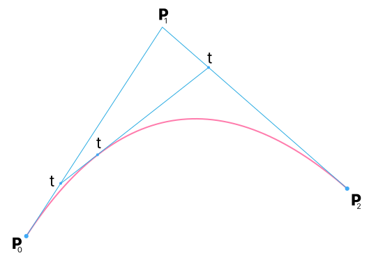
Well, it's a triple linear interpolation, isn't it? The result is the linear interpolation of the linear interpolation between the first end point and the control point and the linear interpolation of the control point and second end point. Given that is true, it can be trivially rephrased as:
$$\begin{split} \mathbf{P}(t) &= (1-t) \left[ (1-t)\mathbf{P_0} + t\mathbf{P_1}\right] + t\left[(1-t)\mathbf{P_0} + t\mathbf{T_0} \right] \\ &= (1-t)^2\mathbf{P_0} + 2(1-t)t\mathbf{P_1} + t^2\mathbf{P_2} \end{split}$$
That is beginning to look an awful lot like the algorithm attributed to de Casteljau. And this is one way of arriving at it that I find particularly intuitive. Rearrangement following the result of an intuitive base assumption. You don't go trying "well, maybe we do triple interpolation" without any real argument to do so. Especially because you need to understand how $t$ plays into it. I mean, you can, but stumbling onto it is not a good look. At least, as far as I'm concerned.
Cubic Bézier curve
If a linear Bézier curve can be represented with a single linear interpolation, a quadratic with three... Well, now we have a leg to stand on and posit that a cubic could be represented with six, using the same tree-like approach! It also stands to reason there will be two control points aiding the two end points:
$$\Large{\begin{split} \mathbf{P}_{0 \rightarrow 1}(t) &= (1-t)\mathbf{P_0} + t\mathbf{P_1} \\ \mathbf{P}_{1 \rightarrow 2}(t) &= (1-t)\mathbf{P_1} + t\mathbf{P_2} \\ \mathbf{P}_{2 \rightarrow 3}(t) &= (1-t)\mathbf{P_2} + t\mathbf{P_3} \\ \end{split}}$$
$$\Large{\begin{split} \mathbf{P}(t) &= (1-t) \left[ (1-t)\mathbf{P}_{0 \rightarrow 1}(t) + t\mathbf{P}_{1 \rightarrow 2}(t)\right] \\ &+ t\left[(1-t)\mathbf{P}_{1 \rightarrow 2}(t) + t\mathbf{P}_{2 \rightarrow 3}(t) \right] \\ \end{split}}$$
Which can be further rearranged and expressed in terms of the points as:
$$\Large{\begin{split} \mathbf{P}(t) = (1-t)^3\mathbf{P_0} &+ 3(1-t)^2t\mathbf{P_1} \\ &+ 3(1-t)t^2\mathbf{P_2} + t^3\mathbf{P_3} \\ \end{split}}$$
Those are some mad binomial expansion vibes. Or, if you have a stronger background in mathematics to contrast against, Bernstein polynomials come to mind. But notice how we didn't need Bernstein polynomials to define the curves underlying all of modern vector graphics. For completeness and generalization, we are going to go there, though.
Deriving Bernstein polynomials to take us the rest of the way
Now is the time to bring up the relationship with Bernstein polynomials. The reason we turn to Bernstein is because his work simplifies our path to generalization. This is motivated by the observation that we can transform our parametric curve equations into the Bernstein form. Don't worry, I'll ease you into it.
Where to begin? Alright, at the end of the 19th century, one very useful mathematical curiousity was whether or not we could approximate any reasonably smooth function with a polynomial to arbitrary precision, whether it is possible to find a polynomial $p(x)$ for which it holds $|f(x) - p(x)| < \epsilon$ for any $x$ on the $[0,1]$ range. The range is sufficient as any function of interest delimited on $[a, b]$ can be translated and scaled to it. The first person to publicly prove this was Weierstrass when he was 70 years old (!), hence why the theorem bears his name.
Sergei Bernstein was a Russian mathematician who lived in a time when today's Stone-Weierstrass theorem was just the Weierstrass theorem and one of his many contributions to mathematics was a probabilistic proof of said theorem in 1912 based on Bernoulli trials, contrasting the constructive one originally proposed by Weierstrass himself. Bernstein argued, in a short one-page paper written in French, that you can subvert the calculation of the expected value of a binomial distribution and the weak law of large numbers in order to prove the Weierstrass theorem.
I have already covered deriving the binomial distribution years ago, which means that you have sufficient information on this website to understand the proof I'm about to outline.
From my other article, or from your past studies, we know that the expected value $\mu$ of the binomial distribution is
$$ \mu = \sum_{k=0}^{n} { k \space {n \choose k} x^k(1-x)^{n-k} } = nx$$
As it is a discrete distribution, another little, however obvious, tidbit is important to explicitly note:
$$ \sum_{k=0}^{n} { \space {n \choose k} x^k(1-x)^{n-k} } = 1$$
Why is this relevant here? Because we can then setup $p(x)$ as
$$ p(x) = E_n = \sum_{k=0}^{n} { f\left(\frac{k}{n}\right) {n \choose k} x^k(1-x)^{n-k} }$$
and the following will be valid
$$\large{ f(x) - p(x) = \sum_{k=0}^{n} { \left[f(x) - f\left(\frac{k}{n}\right)\right] {n \choose k} x^k(1-x)^{n-k} }}$$
When $k/n$ is close to $x$, the $E_n$ above clearly approximates $f(x)$. What about everywhere else? A well-behaved function has a global maximum $M$ on any delimited range, the worst case scenario is that our $p(x)$ will miss by a maximum of $2M$. Why twice the global maximum? Imagine being at the sea floor (below sea level, yes?) looking up at a mountain. $2M$. At worst, $M$ to clear the sea and $M$ to reach the top of the mountain.
How do we quantify these conditions? We split the problem on $x$. Continuity of the function guarantees that we can define the values $\epsilon$ and $\delta$ as
$$ |x - x'| \leq \delta \implies |f(x) - f(x')| < \epsilon/2 $$
We can restate it in terms of the maximum $f_{M}(x)$ and the minimum $f_{m}(x)$, defined on the interval $(x - \delta, x + \delta)$. It trivially follows that $f_{M}(x) - f(x) < \epsilon/2$ and $f(x) - f_{M}(x) < \epsilon/2$. Armed with these relations, we can start playing with constraining the expected value (which is $p(x)$ aliased as $E_n$). There's two outcomes, $|x - k/n| < \delta$ and $|x - k/n| \geq \delta$. The expected value is, therefore, constrained by the weighted average of the two on both ends, weight being the probability $q$ that $|x - k/n| \geq \delta$:
$$ (1-q)f_{m}(x) - qM < p(x) < (1-q)f_{M}(x) + qM$$
Now, that $n$ in the denominator comes handy. We can push $n$ so high that $q$ dwindles to a point where it'll be smaller than our carefully chosen constraint of $\epsilon/(4M)$. If you expand the previous equation's minimum and maximum expressions in terms of $f(x)$ and replace $q$ with our constraint, everything collapses to
$$ f(x) - \frac{\epsilon}{2} - \frac{2M}{4M}\epsilon < p(x) < f(x) + \frac{\epsilon}{2} + \frac{2M}{4M}\epsilon.$$
Cancel, combine and cleanup to recover the expected inequality
$$ |f(x) - p(x)| < \epsilon.$$
This concludes the proof.
On proving Weierstrass' theorem
This section warrants its own article with significantly more detail, possibly even covering multiple approaches, however, I cannot be bothered right now.
From the result of the proof, it becomes obvious that the mathematical foundation of the binomial distribution can be transformed into basis functions which, when linearly combined with coefficients, are capable of approximating any well-behaved function. Bernstein polynomials can therefore be defined implicitly as:
$$ p(x) = \sum_{k=0}^{n} { a_k b_{n,k}(x) } = \sum_{k=0}^{n} { a_k {n \choose k} x^k(1-x)^{n-k} }$$
$n$-choose-$k$ may obscure the fact that the following is true:
$$ \mathbf{P}(t) = \sum_{k=0}^{n=2} { \mathbf{P}_k b_{n,k}(t) } = (1-t)^2\mathbf{P_0} + 2(1-t)t\mathbf{P_1} + t^2\mathbf{P_2}$$
Obviously, it works for the linear case as well:
$$ \mathbf{P}(t) = \sum_{k=0}^{n=1} { \mathbf{P}_k b_{n,k}(t) } = (1-t)\mathbf{P_0} + t\mathbf{P_1}$$
As it does for the cubic, the quartic and the $n$-th degree curve case. If you feel like it, work them out. You don't really need more than quadratic and cubic curves in practice, in the field of vector graphics at least.